By Eric Gregori
Senior Software Engineer
BDTI
This article was originally published at EE Times' Embedded.com Design Line. It is reprinted here with the permission of EE Times.
The term “embedded vision” refers to the use of computer vision technology in embedded systems. Stated another way, “embedded vision” refers to embedded systems that extract meaning from visual inputs.
Similar to the way that wireless communication has become pervasive over the past 10 years, embedded vision technology is poised to be widely deployed in the next 10 years. Vision algorithms were originally only capable of being implemented on costly, bulky, power-hungry computer systems, and as a result computer vision has mainly been confined to a few application areas, such as factory automation and military equipment.
Today, however, a major transformation is underway. Due to the emergence of very powerful, low-cost, and energy-efficient processors, image sensors, memories and other ICs, it has become possible to incorporate vision capabilities into a wide range of embedded systems.
Similarly, OpenCV, a library of computer vision software algorithms originally designed for vision applications and research on PCs has recently expanded to support embedded processors and operating systems.
Intel started OpenCV in the mid 1990s as a method of demonstrating how to accelerate certain algorithms. In 2000, Intel released OpenCV to the open source community as a beta version, followed by v1.0 in 2006. Robot developer Willow Garage, founded in 2006, took over support for OpenCV in 2008 and immediately released v1.1. The company has been in the news a lot lately, subsequent to the unveiling of its PR2 robot.
OpenCV v2.0, released in 2009, contained many improvements and upgrades. Initially, the majority of algorithms in the OpenCV library were written in C, and the primary method of using the library was via a C API. OpenCV v2.0 migrated towards C++ and a C++ API. Subsequent versions of OpenCV added Python support, along with Windows, Linux, iOS and Android OS support, transforming OpenCV (currently at v2.3) into a cross-platform tool. OpenCV v2.3 contains more than 2,500 functions.
What can you do with OpenCV v2.3? Think of OpenCV as a box of 2,500 different food items. The chef's job is to combine the food items into a meal. OpenCV in itself is not the full meal; it contains the pieces required to make a meal. But the good news is that OpenCV includes a suite of recipes that provide examples of what it can do.
Experimenting with OpenCV
If you’d like to quickly do some hands-on experimentation with basic computer vision algorithms, without having to install any tools or do any programming, you’re in luck. BDTI has created the BDTI OpenCV Executable Demo Package, an easy-to-use software package that allows anyone with a Windows computer and a web camera to run a set of interactive computer vision algorithm examples built with OpenCV v2.3.
You can download the installer zip file from the Embedded Vision Alliance website, in the Embedded Vision Academy section (free registration is required). The installer will place several prebuilt OpenCV applications on your computer, and you can run the examples directly from your Start menu. BDTI has also developed an online user guide and tutorial video for the OpenCV demonstration package.
Examples named xxxxxxSample.bat use a video clip file as an input (example video clips are provided with the installation), while examples named xxxxxWebCamera.bat use a video stream from a web camera as an input. BDTI will periodically expand the BDTI OpenCV Executable Demo Package with additional OpenCV examples; keep an eye on the Embedded Vision Academy section of the Embedded Vision Alliance website for updates.
Developing Apps with OpenCV
The most difficult part of using OpenCV is building the library and configuring the tools. The OpenCV development team has made great strides in simplifying the OpenCV build process, but it can still be time consuming.
To make it as easy as possible to start using OpenCV, BDTI has also created the BDTI Quick-Start OpenCV Kit – a VMware virtual machine image that includes OpenCV and all required tools preinstalled, configured, and built. The BDTI Quick-Start OpenCV Kit makes it easy to quickly get OpenCV running and to start developing vision algorithms using OpenCV.
The BDTI Quick-Start OpenCV Kit image uses Ubuntu 10.04 as the operating system (Figure 1 below). The associated Ubuntu desktop is intuitive and easy to use. OpenCV 2.3.0 has been preinstalled and configured in the kit, along with the GNU C compiler and tools (GCC version 4.4.3). Various examples are included, along with a framework so you can get started creating your own vision algorithms immediately.
The Eclipse integrated development environment is also installed and configured for debugging OpenCV applications. Various Eclipse OpenCV examples are included to get you up and running quickly and to seed your own projects. And four example Eclipse projects are provided to seed your own projects.
Figure 1: The Ubuntu Desktop installed in the BDTI VMware virtual machine image
A USB webcam is required to use the examples provided in the BDTI Quick-Start OpenCV Kit. Logitech USB web cameras, specifically the Logitech C160 in conjunction with the free VMware Player for Windows and VMware Fusion for Mac OS X, have been tested with this virtual machine image. Be sure to install the drivers provided with the camera in Windows or whatever other operating system you use.
To get started, download the BDTI Quick-Start OpenCV Kit from the Embedded Vision Academy area of the Embedded Vision Alliance website (free registration required). BDTI has also created an online user guide for the Quick-Start OpenCV Kit.
OpenCV Examples
Two sets of OpenCV example programs are included in the BDTI Quick-Start OpenCV Kit. The first set is command-line based, the second set is Eclipse IDE based.
The command line examples include example makefiles to provide guidance for your own projects. The Eclipse examples are the same as the command-line examples but configured to build in the Eclipse environment. The source code is identical, but the makefiles are specialized for building OpenCV applications in an Eclipse environment.
The same examples are also provided in the previously mentioned BDTI OpenCV Executable Demo Package. Embedded vision involves, among other things, classifying groups of pixels in an image or video stream as either background or a unique feature.
Each of the examples demonstrates various algorithms that accomplish this goal using different techniques. Some of them use code derived from the book OpenCV 2 Computer Vision Application Programming Cookbook by Robert Laganiere (ISBN-10: 1849513244, ISBN-13: 978-1849513241).
A Motion Detection Example
As the name implies, motion detection uses the differences between successive frames to classify pixels as unique features (Figure 2 below). The algorithm considers pixels that do not change between frames as being stationary and therefore part of the background. Motion detection or background subtraction is a very practical and easy-to-implement algorithm.
In its simplest form, the algorithm looks for differences between two frames of video by subtracting one frame from the next. In the output display in this example, white pixels are moving, black pixels are stationary.
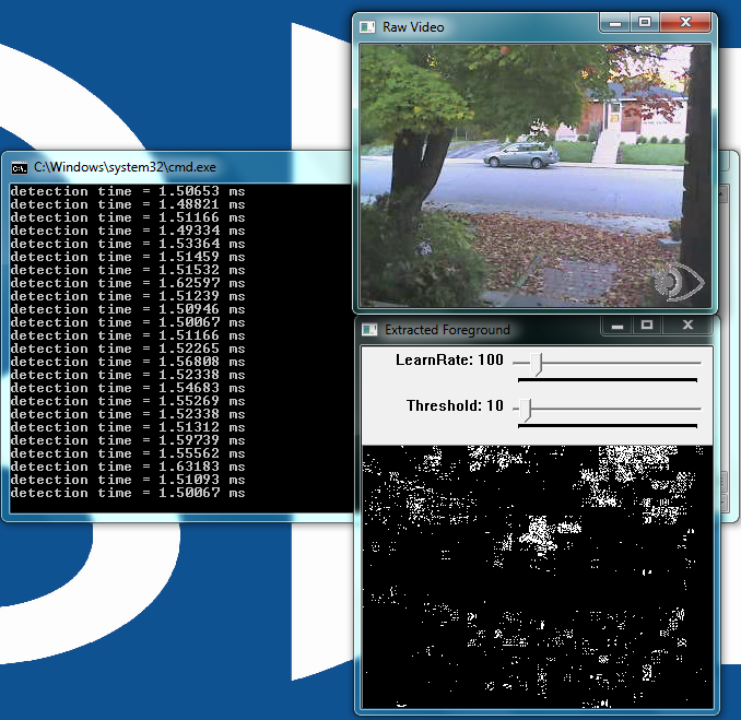
Figure 2: The user interface for the motion detection example, included in both the BDTI OpenCV Executable Demo Package (top) and the BDTI Quick-Start OpenCV Kit (bottom)
This example adds an additional element to the simple frame subtraction algorithm: a running average of the frames.The number of frames in the running average represents a length in time.
The LearnRate sets how fast the accumulator “forgets” about earlier images. The higher the LearnRate, the longer the running average. By setting LearnRate to 0, you disable the running average and the algorithm simply subtracts one frame from the next.[JB2] Increasing the LearnRate is useful for detecting slow moving motion.
The Threshold parameter sets the change level required for a pixel to be considered moving. The algorithm subtracts the current frame from the previous frame, giving a result. If the result is greater than the threshold, the algorithm displays a white pixel and considers that pixel to be moving.
Variables:
- LearnRate: Regulates the update speed (how fast the accumulator "forgets" about earlier images).
- Threshold: The minimum value for a pixel difference to be considered moving.
The Line Detection Example
Line detection classifies straight edges in an image as features (Figure 3 below). The algorithm relegates to the background anything in the image that it does not recognize as a straight edge, thereby ignoring it. Edge detection is another fundamental function in computer vision.
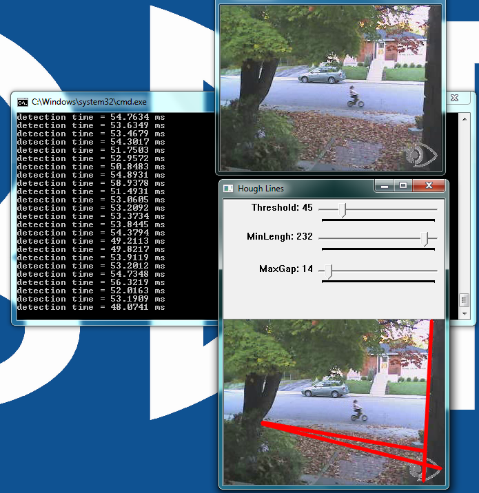
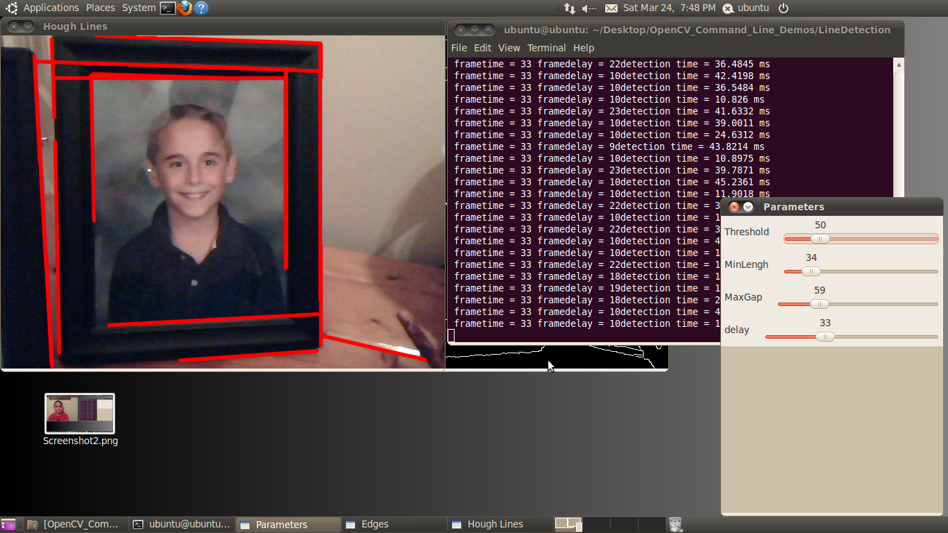
Figure 3: The user interface for the line detection example, included in both the BDTI OpenCV Executable Demo Package (top) and the BDTI Quick-Start OpenCV Kit (bottom)
Image processing determines an edge by sensing close-proximity pixels of differing intensity. For example, a black pixel next to a white pixel defines a “hard” edge. A gray pixel next to a black (or white) pixel defines a “soft” edge.
The Threshold parameter sets a minimum on how hard an edge has to be in order for it to be classified as an edge. A Threshold of 255 would require a white pixel be next to a black pixel to qualify as an edge. As the Threshold value decreases, softer edges in the image are detected.
After the algorithm detects an edge, it must make a difficult decision: is this edge part of a straight line? The Hough transform, employed to make this decision, attempts to group pixels classified as edges into a straight line.
It uses the MinLength and MaxGap parameters to decide ("classify" in computer science lingo) a group of edge pixels into either a straight continuous line or ignored background information (edge pixels not part of a continuous straight line are considered background, and therefore not a feature).
Variables:
- Threshold: Sets the minimum difference between adjacent pixels to be classified as an edge.
- MinLength: The minimum number of "continuous" edge pixels required to classify a potential feature as a straight line.
- MaxGap: The maximum allowable number of missing edge pixels that still enable classification of a potential feature as a "continuous" straight line.
The Optical Flow Example
Optical flow estimates motion by analyzing how groups of pixels in the current frame changed position from the previous frame of a video sequence (Figure 4 below).
The "group of pixels" is a feature. Optical flow estimation finds use in predicting where objects will be in the next frame. Many optical flow estimation algorithms exist; this particular example uses the Lucas-Kanade approach. The algorithm's first step involves finding "good" features to track between frames. Specifically, the algorithm is looking for groups of pixels containing corners or points.
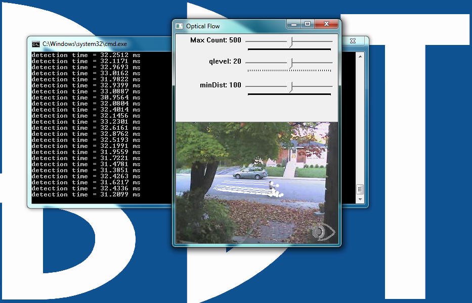
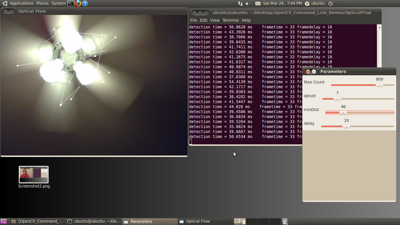
Figure 4: The user interface for the optical flow example, included in both the BDTI OpenCV Executable Demo Package (top) and the BDTI Quick-Start OpenCV Kit (bottom)
The qlevel variable determines the quality of a selected feature. Consistency is the end objective of using a lot of math to find quality features.
A "good" feature (group of pixels surrounding a corner or point) is one that an algorithm can find under various lighting conditions, as the object moves. The goal is to find these same features in each frame.
Once the same feature appears in consecutive frames, tracking an object is possible. The lines in the output video represent the optical flow of the selected features.
The MaxCount parameter determines the maximum number of features to look for. The minDist parameter sets the minimum distance between features. The more features used, the more reliable the tracking.
The features are not perfect, and sometimes a feature used in one frame disappears in the next frame. Using multiple features decreases the chances that the algorithm will not be able to find any features in a frame.
Variables:
- MaxCount: The maximum number of good features to look for in a frame.
- qlevel: The acceptable quality of the features. A higher quality feature is more likely to be unique, and therefore to be correctly identified in the next frame. A low quality feature may get lost in the next frame, or worse yet may be confused with another feature in the image of the next frame.
- minDist: The minimum distance between selected features.
The Face Detector Example
The face detector used in this example is based on the Viola-Jones feature detector algorithm (Figure 5 below). Throughout this article, we have been working with different algorithms for finding features; i.e. closely grouped pixels in an image or frame that are unique in some way.
The motion detector used subtraction of one frame from the next frame to find pixels that moved, classifying these pixel groups as features. In the line detector example, features were groups of edge pixels organized in a straight line. And in the optical flow example, features were groups of pixels organized into corners or points in an image.
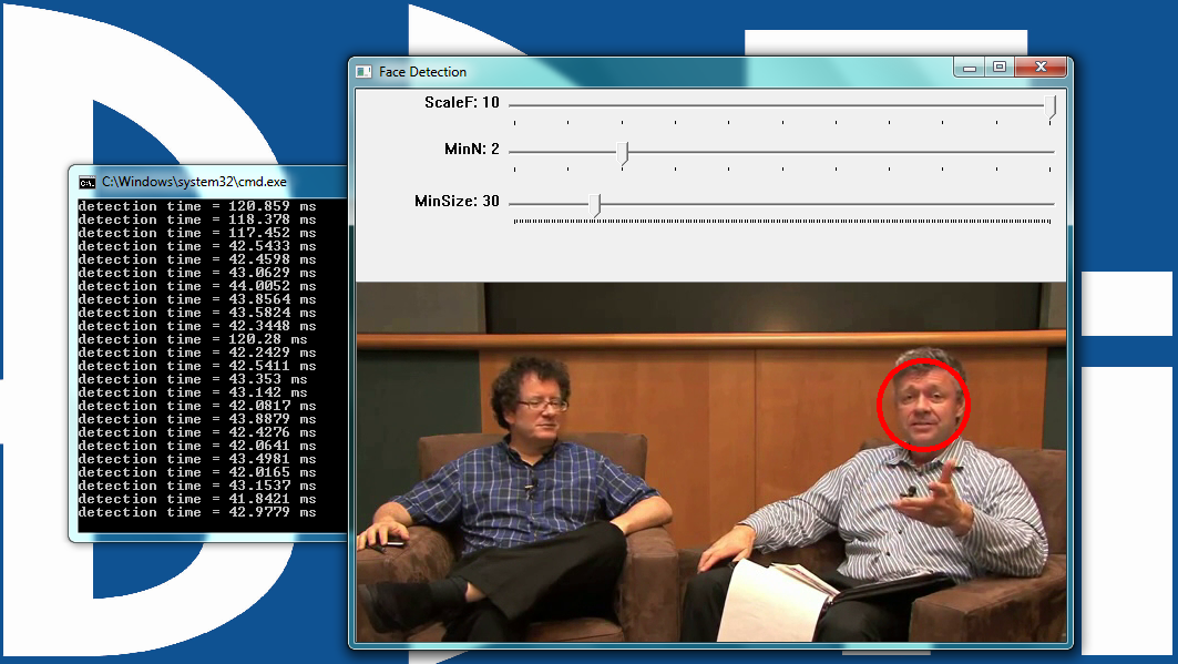
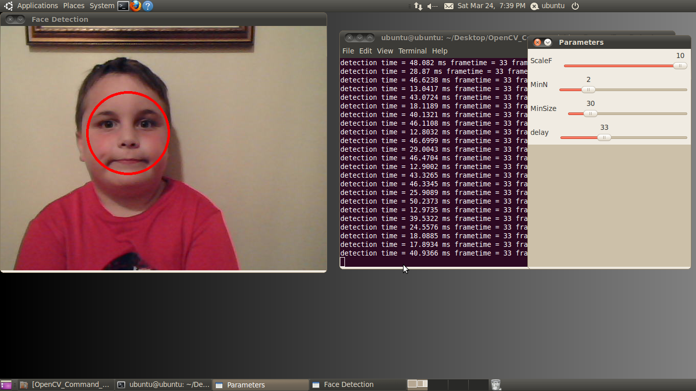
Figure 5: The user interface for the face detector example, included in both the BDTI OpenCV Executable Demo Package (top) and the BDTI Quick-Start OpenCV Kit (bottom)
The Viola-Jones algorithm uses a discrete set of six Haar-like features (the OpenCV implementation adds additional features). Haar-like features in a 2D image include edges, corners, and diagonals. They are very similar to features in the optical flow example, except that detection of these particular features occurs via a different method.
As the name implies, the face detector example detects faces. Detection occurs within each individual frame; the detector does not track the face from frame to frame.
The face detector can also detect objects other than faces. An XML file "describes" the object to detect. OpenCV includes various Haar cascade XML files that you can use to detect various object types. OpenCV also includes tools to allow you to train your own cascade to detect any object you desire and save it as an XML file for use by the detector.
Variables:
- MinSize: The smallest face to detect. As a face gets further from the camera, it appears smaller. This parameter also defines the furthest distance a face can be from the camera and still be detected.
- MinN: The “minimum neighbor” parameter combines, into a single detection, faces that are detected multiple times. The face detector actually detects each face multiple times in slightly different positions. This parameter simply defines how to group the detections together. For example, a MinN of 20 would group all detection within 20 pixels of each other as a single face.
- ScaleF: Scale factor determines the number of times to run the face detector at each pixel location. The Haar cascade XML file that determines the parameters of the to-be-detected object is designed for an object of only one size.
In order to detect objects of various sizes (faces close to the camera as well as far away from the camera, for example) requires scaling the detector.
This scaling process has to occur at every pixel location in the image. This process is computationally expensive, but a scale factor that is too large will not detect faces between detector sizes.
A scale factor too small, conversely, can use a huge amount of CPU resources. You can see this phenomenon in the example if you first set the scale factor to its max value of 10. In this case, you will notice that as each face moves closer to or away from the camera, the detector will not detect it at certain distances.
At these distances, the face size is in-between detector sizes. If you decrease the scale factor to its minimum, on the other hand, the required CPU resources skyrocket, as shown by the prolonged detection time.
Detection Time Considerations
Each of these examples writes the detection time to the console while the algorithm is running. This time represents the number of milliseconds the particular algorithm took to execute.
A larger amount of time represents higher CPU utilization. The OpenCV library as built in these examples does not have hardware acceleration enabled; however OpenCV currently supports CUDA and NEON acceleration.
The intent of this article and accompanying software is to help you quickly get up and running with OpenCV. The examples discussed in this article represent only a miniscule subset of algorithms available in OpenCV; they were chosen because at a high level they represent a broad variety of computer vision functions.
Leveraging these algorithms in combination with, or alongside, other algorithms can help you solve various embedded vision problems in a variety of applications.
Stay tuned for future articles in this series on Embedded.com, which will both go into more detail on already-mentioned OpenCV library algorithms and introduce new algorithms (along with the BDTI OpenCV Executable Demo Package and the BDTI Quick-Start OpenCV Kit -based examples of the algorithms).
Conclusion
Embedded vision technology has the potential to enable a wide range of electronic products that are more intelligent and responsive than before, and thus more valuable to users. It can add helpful features to existing products.
And it can provide significant new markets for hardware, software and semiconductor manufacturers. The Embedded Vision Alliance, a worldwide organization of technology developers and providers of which BDTI is a founding member, is working to empower engineers to transform this potential into reality in a rapid and efficient manner.
More specifically, the mission of the Alliance is to provide engineers with practical education, information, and insights to help them incorporate embedded vision capabilities into products.
To execute this mission, the Alliance has developed a full-featured website, freely accessible to all and including (among other things) articles, videos, a daily news portal and a discussion forum staffed by a diversity of technology experts.
Registered website users can receive the Embedded Vision Alliance's e-mail newsletter; they also gain access to the Embedded Vision Academy, containing numerous training videos, technical papers and file downloads, intended to enable those new to the embedded vision application space to rapidly ramp up their expertise.
Eric Gregori is a Senior Software Engineer and Embedded Vision Specialist with Berkeley Design Technology, Inc. (BDTI), which povides analysis, advice, and engineering for embedded processing technology and applications. He is a robot enthusiast with over 17 years of embedded firmware design experience, with specialties in computer vision, artificial intelligence, and programming for Windows Embedded CE, Linux, and Android operating systems. Eric authored the Robot Vision Toolkit and developed the RobotSee Interpreter. He is working towards his Masters in Computer Science and holds 10 patents in industrial automation and control.
(Editor’s Note: The Embedded Vision Alliance was launched in May of 2011, and now has 19 sponsoring member companies: AMD, Analog Devices, Apical, Avnet Electronics Marketing, BDTI, CEVA, Cognimem, CogniVue, eyeSight, Freescale, IMS Research, Intel, MathWorks, Maxim Integrated Products, NVIDIA, National Instruments, Omek Interactive, Texas Instruments, Tokyo Electron Device, and Xilinx.
The first step of the Embedded Vision Alliance was to launch a website at www.Embedded-Vision.com. The site serves as a source of practical information to help design engineers and application developers incorporate vision capabilities into their products. The Alliance’s plans include educational webinars, industry reports, and other related activities.
Everyone is free to access the resources on the website, which is maintained through member and industry contributions. Membership details are also available at the site. For more information, contact the Embedded Vision Alliance at [email protected] and 1-510-451-1800.)