OpenCV is an open-source software component library for computer vision application development. OpenCV is a powerful tool for prototyping embedded vision algorithms. Originally released in 2000, it has been downloaded over 3.5 million times. The OpenCV library supports over 2,500 functions and contains dozens of valuable vision application examples. The library supports C, C++, and Python and has been ported to Windows, Linux, Android, MAC OS X and iOS.
The most difficult part of using OpenCV is building the library and configuring the tools. The OpenCV development team has made great strides in simplifying the OpenCV build process, but it can still be time consuming. To make it as easy as possible to start using OpenCV, BDTI has created the Quick-Start OpenCV Kit, a VMware image that includes OpenCV and all required tools preinstalled, configured, and built. This makes it easy to quickly get OpenCV running and to start developing vision algorithms using OpenCV. The BDTI Quick-Start OpenCV Kit can be run on any Windows computer by using the free VMware player, or on Mac OS X using VMware Fusion. This article describes the process of installing and using the BDTI Quick-Start OpenCV Kit. For more information about OpenCV and other OpenCV tools from BDTI, go here.
Please note that the BDTI Quick-Start OpenCV Kit contains numerous open source software packages, each with its own license terms. Please refer to the licenses associated with each package to understand what uses are permitted. If you have questions about any of these licenses, please contact the authors of the package in question. If you believe that the BDTI OpenCV VMware image contains elements that should not be distributed in this way, please contact us.
Figure 1. Ubuntu desktop installed in the BDTI VMware image
The BDTI Quick-Start OpenCV Kit uses Ubuntu 10.04 for the OS. The Ubuntu desktop is intuitive and easy to use. OpenCV 2.3.0 has been preinstalled and configured in the image, along with the GNU C compiler and tools (gcc version 4.4.3). Various examples are included along with a framework so you can get started with your own vision algorithms immediately. The Eclipse integrated development environment is also installed and configured for debugging OpenCV applications. Five example Eclipse projects are included to seed your own projects.
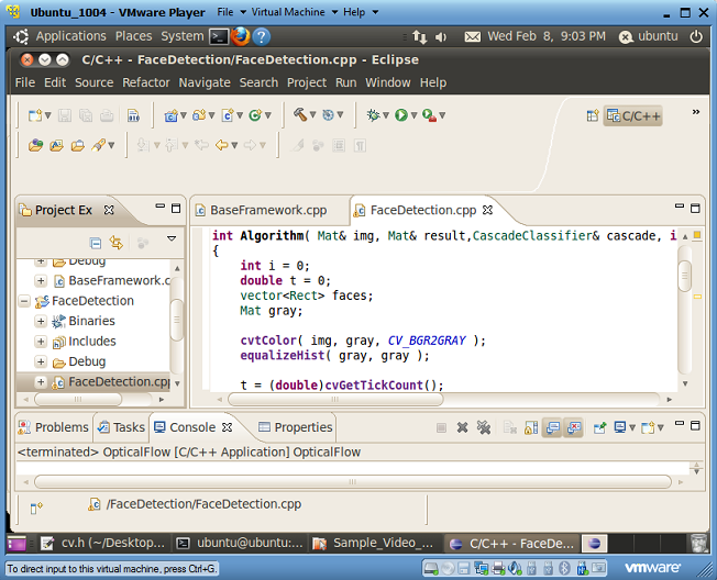
Figure 2. Eclipse integrated development environment installed in the BDTI VMware image
A USB webcam is required to use the examples provided in the BDTI Quick-Start OpenCV Kit. Logitech USB web cameras have been tested with this image, specifically the Logitech C160. Be sure to install the Windows drivers provided with the camera on your Windows system.
To get started, first download the BDTI Quick-Start OpenCV Kit from the Embedded Vision Academy. To use the image on Windows, you must also download the free VMware player. After downloading the zip file from the Embedded Vision Academy, unzip it into a folder. Double-click the vmx file highlighted by the arrow in Figure 3. If you have VMware player correctly installed, you should see the Ubuntu desktop as shown in Figure 1. You may see some warnings upon opening the VMware image concerning “Removable Devices.” If so, simply click “OK.” In addition, depending on which version of VMware player you have, you may get a window concerning “Software Updates.” Simply click “Remind Me Later.”
Figure 3. The unzipped BDTI OpenCV VMware image
To shut down the VMware image, click the “power button” in the upper right corner of the Ubuntu desktop and select “Shut Down.”
To connect the webcam to the VMware image, plug the webcam into your computer’s USB port and follow the menus shown in Figure 4. Find the “Virtual Machine” button in the top of the VMware window as shown highlighted in Figure 4. Then select “Removable Devices” and look for your webcam in the list. Select your webcam and click connect. For correct operation your webcam should have a check mark next to it, as shown by the Logitech USB device (my web camera) in Figure 4.
Figure 4. Connecting the camera to the VMware image
To test your camera with the VMware image, double click the “Click_Here_To_Test_Your_Camera” icon in the upper left corner of the Ubuntu Desktop. A window should open showing a live feed from the camera. If you do not see a live video feed, verify that the camera is connected to the VMware image using the menus shown in Figure 4. If the camera is still not working, exit the VMware image and try the camera on the Windows host. The camera must be properly installed on the Windows host per the manufacturer’s instructions.
Command Line OpenCV Examples
There are two sets of OpenCV examples preloaded in the BDTI Quick-Start OpenCV Kit. The first set is command-line based, the second set is Eclipse IDE based. The command line examples can be found in the “OpenCV_Command_Line_Demos” folder as shown in Figure 5.
Figure 5. OpenCV command line demos folder
Double click the “Terminal” icon and type “. ./demos” at the prompt. That is a period, followed by a space, followed by a period and a forward slash then the word demos. Commands are case sensitive, so watch the Caps Lock key.
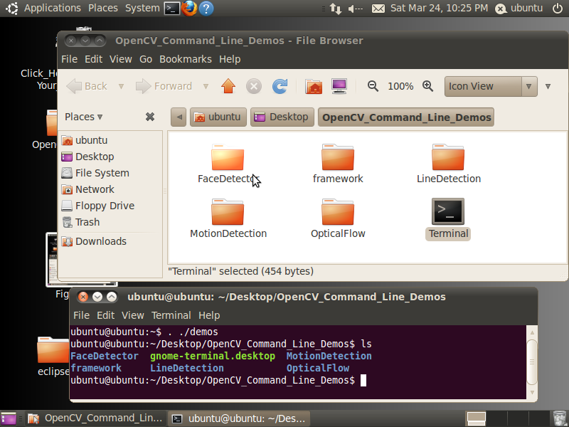
Figure 6. The command line demos
The command line examples include example makefiles to provide guidance for your own projects. To build a demo, simply change directory into the directory for that demo and type “make”, as illustrated here (commands below are in bold):
ubuntu@ubuntu:~/Desktop/OpenCV_Command_Line_Demos$ ls
FaceDetector gnome-terminal.desktop MotionDetection
framework LineDetection OpticalFlow
ubuntu@ubuntu:~/Desktop/OpenCV_Command_Line_Demos$ cd FaceDetector/
ubuntu@ubuntu:~/Desktop/OpenCV_Command_Line_Demos/FaceDetector$ ls
example example.cpp example.o haarcascade_frontalface_alt2.xml Makefile
ubuntu@ubuntu:~/Desktop/OpenCV_Command_Line_Demos/FaceDetector$ make
All of the examples are named “example.cpp” and create an executable binary with name “example”. To run the program, type “./example”.
ubuntu@ubuntu:~/Desktop/OpenCV_Command_Line_Demos/FaceDetector$ ./example
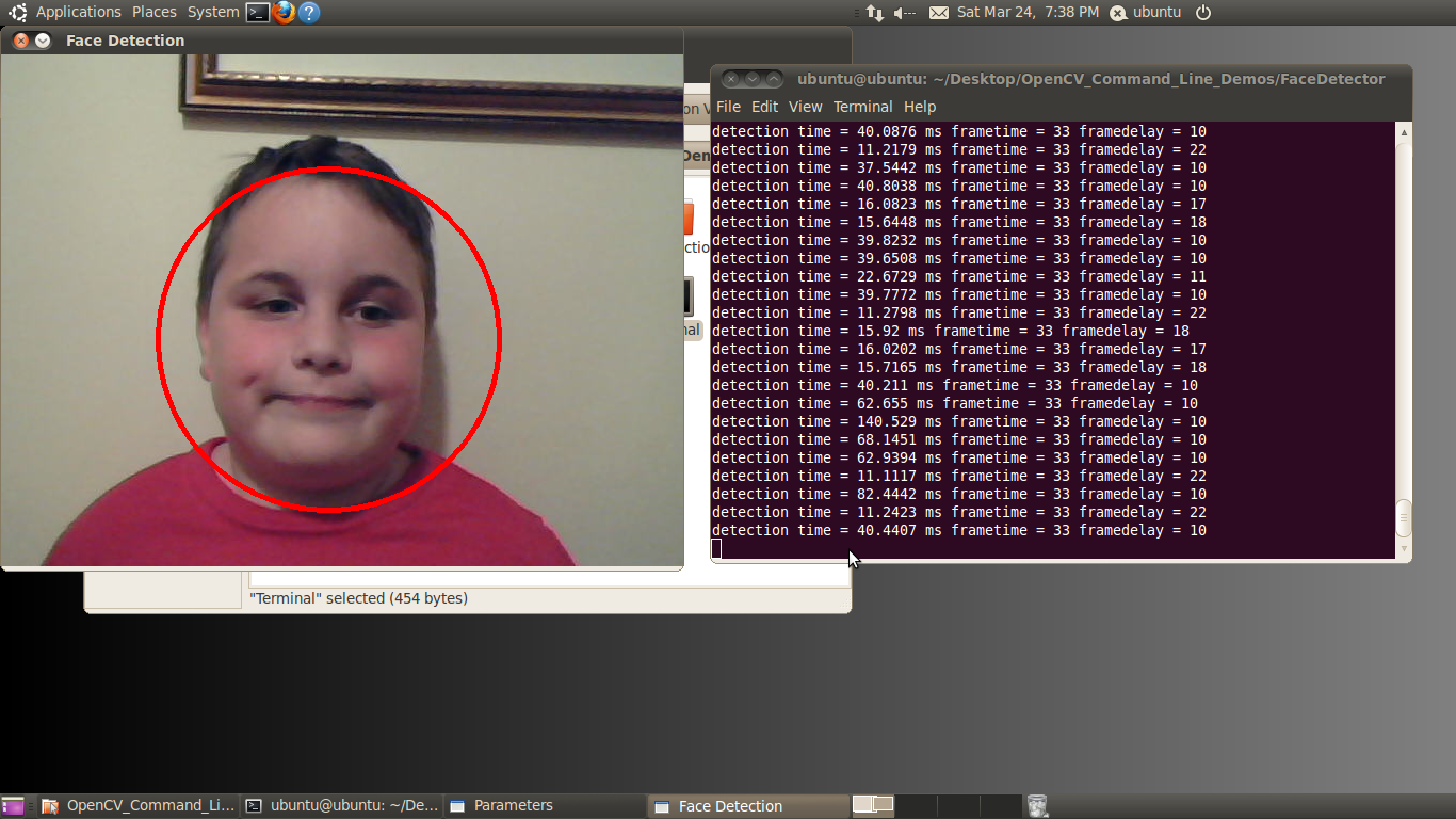
Figure 7. The face detector example
To exit the example, simply highlight the one of the windows (other than the console window) and push any key.
To edit a command line example, use the “gedit” command to launch a graphical editor.
ubuntu@ubuntu:~/Desktop/OpenCV_Command_Line_Demos/FaceDetector$ gedit example.cpp &
This opens the file named “example.cpp” in the graphical editor as shown in Figure 8.
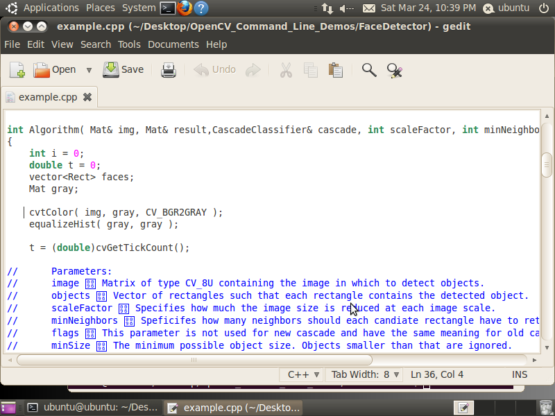
Figure 8. Using gedit to edit an OpenCV example C file
Eclipse Graphical Integrated Development Environment OpenCV Examples
The Eclipse examples are the same as the command line examples but configured to build in the Eclipse environment. The source code is identical, but the makefiles are specialized for building OpenCV applications in an Eclipse environment. To start the Eclipse IDE, double click the “Eclipse_CDT” icon on the Ubuntu Desktop. Eclipse will open as shown in Figure 2.
The left Eclipse pane lists the OpenCV projects. The center pane is the source debugger. To debug a project, simply highlight the desired project in the left pane and click the green bug on the top toolbar. When the debug window opens, push F8 (see Figure 9).
Figure 9. Debugging an OpenCV example in Eclipse
The Eclipse IDE makes it easy to debug your OpenCV application by allowing you to set breakpoints, view variables, and step through code. For more information about debugging with eclipse, read this excellent guide. To stop debugging simply click on the red square in the IDE debugger.
There are five examples, each provided in both the Eclipse and command line build format. These five examples have been chosen to show common computer vision functions in OpenCV. Each example uses OpenCV sliders to control the parameters of the algorithm on the fly. Moving these sliders with your mouse will change the specified parameter in real-time, letting you experiment with the behavior of the algorithm without writing any code. The five examples are motion detection, line detection, optical flow and face detection. Each is described briefly below. This article does not go into details of each algorithm; look for future articles covering each of the algorithms used in these examples in detail. For now, let’s get to the examples.
Motion Detection
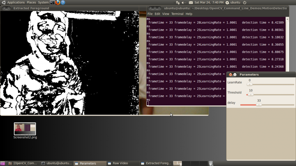
As the name implies, motion detection uses the change of pixels between frames to classify pixels as unique features (Figure 10). The algorithm considers pixels that do not change between frames as being stationary and therefore part of the background. Motion detection or background subtraction is a very practical and easy-to-implement algorithm. In its simplest form, the algorithm looks for differences between two frames of video by subtracting one frame from the next. In the output display, white pixels are moving, black pixels are stationary.
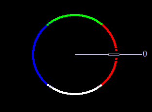
Figure 10. The user interface for the motion detection example
This example adds an additional element to the simple frame subtraction algorithm: a running average of the frames. Each frame averaging routine runs over a time period specified by the LearnRate parameter. The higher the LearnRate, the longer the running average. By setting LearnRate to 0, you disable the running average and the algorithm simply subtracts one frame from the next.
The Threshold parameter sets the change level required for a pixel to be considered moving. The algorithm subtracts the current frame from the previous frame, giving a result. If the result is greater than the threshold, the algorithm displays a white pixel and considers that pixel to be moving.
LearnRate: Regulates the update speed (how fast the accumulator "forgets" about earlier images).
Threshold: The minimum value for a pixel difference to be considered moving.
Line Detection
Line detection classifies straight edges in an image as features (Figure 11). The algorithm relegates to the background anything in the image that it does not recognize as a straight edge, thereby ignoring it. Edge detection is another fundamental function in computer vision.
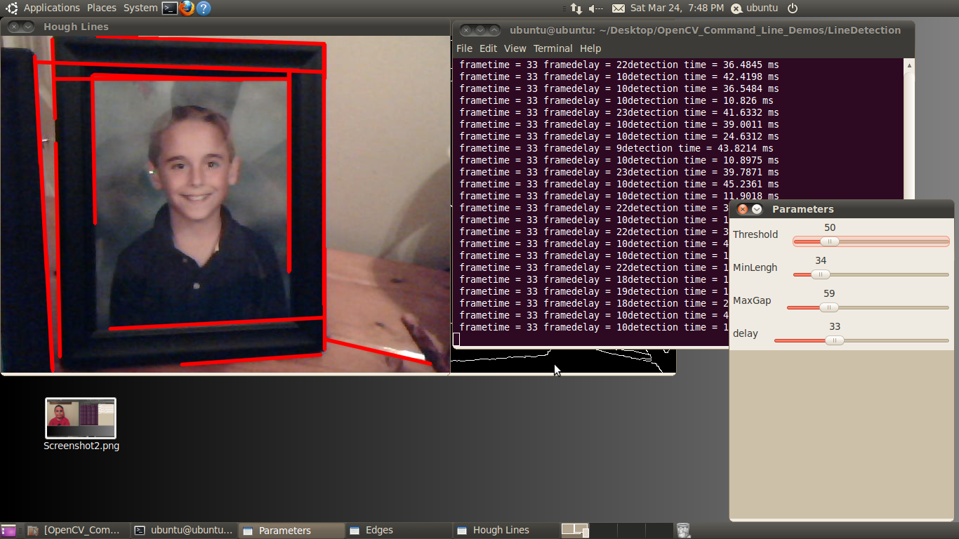
Figure 11. The user interface for the line detection example
Image processing determines an edge by sensing close-proximity pixels of differering intensity. For example, a black pixel next to a white pixel defines a hard edge. A gray pixel next to a black (or white) pixel defines a soft edge. The Threshold parameter sets a minimum on how hard an edge has to be in order for it to be classified as an edge. A Threshold of 255 would require a white pixel be next to a black pixel to qualify as an edge. As the Threshold value decreases, softer edges in the image appear in the display.
After the algorithm detects an edge, it must make a difficult decision: is this edge part of a straight line? The Hough transform, employed to make this decision, attempts to group pixels classified as edges into a straight line. It uses theMinLength and MaxGap parameters to decide ("classify" in computer science lingo) a group of edge pixels into either a straight continuous line or ignored background information (edge pixels not part of a continuous straight line are considered background, and therefore not a feature).
Threshold: Sets the minimum difference between adjoining groups of pixels to be classified as an edge.
MinLength: The minimum number of "continuous" edge pixels required to classify a potential feature as a straight line.
MaxGap: The maximum allowable number of missing edge pixels that still enable classification of a potential feature as a "continuous" straight line.
Optical Flow
Optical flow estimates motion by analyzing how groups of pixels in the current frame changed position from the previous frame of a video sequence (Figure 12). The "group of pixels" is a feature. Optical flow estimation finds use in predict where objects will be in the next frame. Many optical flow estimation algorithms exist; this particular example uses the Lucas-Kanade approach. The algorithm's first step involves finding "good" features to track between frames. Specifically, the algorithm is looking for groups of pixels containing corners or points.
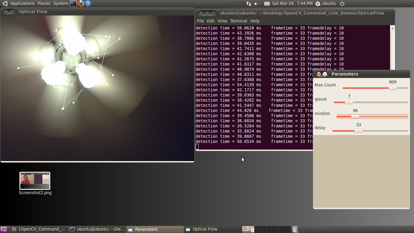
Figure 12. The user interface for the optical flow example
The qlevel variable determines the quality of a selected feature. Consistency is the end objective of using a lot of math to find quality features. A "good" feature (group of pixels surrounding a corner or point) is one that an algorithm can find under various lighting conditions, as the object moves. The goal is to find these same features in each frame. Once the same feature appears in consecutive frames, tracking an object is possible. The lines in the output video represent the optical flow of the selected features.
The MaxCount parameter determines the maximum number of features to look for. The minDist parameter sets the minimum distance between features. The more features used, the more reliable the tracking. The features are not perfect, and sometimes a feature used in one frame disappears in the next frame. Using multiple features decreases the chances that the algorithm will not be able to find any features in a frame.
MaxCount: The maximum number of good features to look for in a frame.
qlevel: The acceptable quality of the features. A higher quality feature is more likely to be unique, and therefore to be correctly findable in the next frame. A low quality feature may get lost in the next frame, or worse yet may be confused with another point in the image of the next frame.
minDist: The minimum distance between selected features.
Face Detector
The face detector used in this example is based on the Viola-Jones feature detector algorithm (Figure 13). Throughout this article, we have been working with different algorithms for finding features; i.e. closely grouped pixels in an image or frame that are unique in some way. The motion detector used subtraction of one frame from the next frame to find pixels that moved, classifying these pixel groups as features. In the line detector example, features were groups of pixels organized in a straight line. And in the optical flow example, features were groups of pixels organized into corners or points in an image.
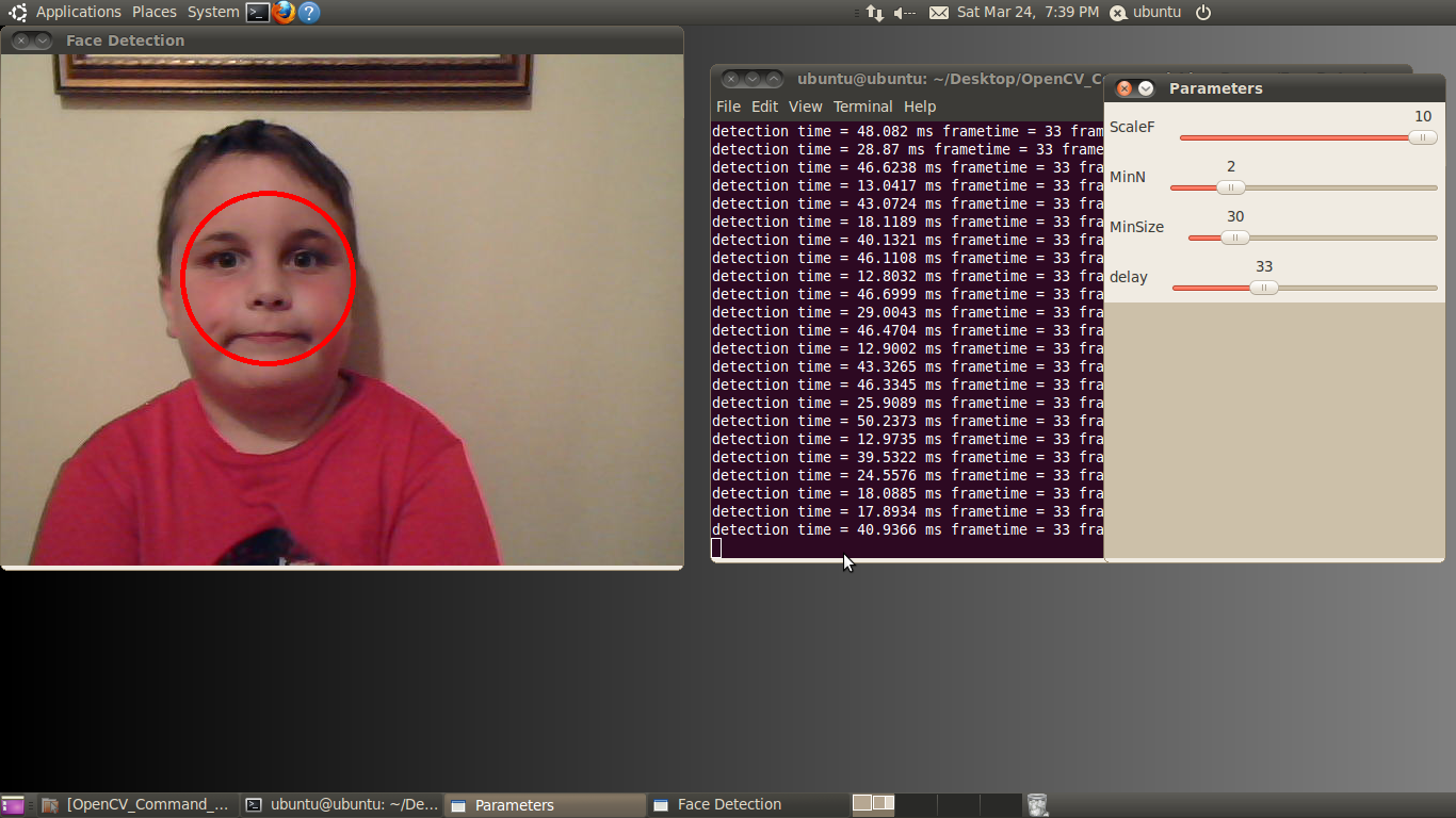
Figure 13. The user interface for the face detector example
The Viola-Jones algorithm uses a discrete set of six Haar-like features (the OpenCV implementation adds additional features). Haar-like features in a 2D image include edges, corners, and diagonals. They are very similar to features in the optical flow example, except that detection of these particular features occurs via a different method.
As the name implies, the face detector example detects faces. Detection occurs within each individual frame; the detector does not track the face from frame to frame. The face detector can also detect objects other than faces. An XML file "describes" the object to detect. OpenCV includes various Haar cascade XML files that you can use to detect various object types. OpenCV also includes tools to allow you to train your own cascade to detect any object you desire and save it as an XML file for use by the detector.
MinSize: The smallest face to detect. As a face gets further from the camera, it appears smaller. This parameter also defines the furthest distance a face can be from the camera and still be detected.
MinN: The minimum neighbor parameter groups faces that are detected multiple times into one detection. The face detector actually detects each face multiple times in slightly different positions. This parameter simply defines how to group the detections together. For example, a MinN of 20 would group all detection within 20 pixels of each other as a single face.
ScaleF: Scale factor determines the number of times to run the face detector at each pixel location. The Haar cascade XML file that determines the parameters of the to-be-detected object is designed for an object of only one size. In order to detect objects of various sizes (faces close to the camera as well as far away from the camera, for example) requires scaling the detector. This scaling process has to occur at every pixel location in the image. This process is computationally expensive, but a scale factor that is too large will not detect faces between detector sizes. A scale factor too small, conversely, can use a huge amount of CPU resources. You can see this phenomenon in the example if you first set the scale factor to its max value of 10. In this case, you will notice that as each face moves closer to or away from the camera, the detector will not detect it at certain distances. At these distances, the face size is in-between detector sizes. If you decrease the scale factor to its minimum, on the other hand, the required CPU resources skyrocket, as shown by the extended detection time.
Canny Edge Detector
Many algorithms exist for finding edges in an image. This example focuses on the Canny algorithm (Figure 14). Considered by many to be the best edge detector, the Canny algorithm was developed in 1986 by John F. Canny of U.C. Berkeley. In his paper, "A computational approach to edge detection," Canny describes three criteria to evaluate the quality of edge detection:
- Good detection: There should be a low probability of failing to mark real edge points, and low probability of falsely marking non-edge points. This criterion corresponds to maximizing signal-to-noise ratio.
- Good localization: The points marked as edge points by the operator should be as close as possible to the center of the true edge.
- Only one response to a single edge: This criterion is implicitly also captured in the first one, since when there are two responses to the same edge, one of them must be considered false.
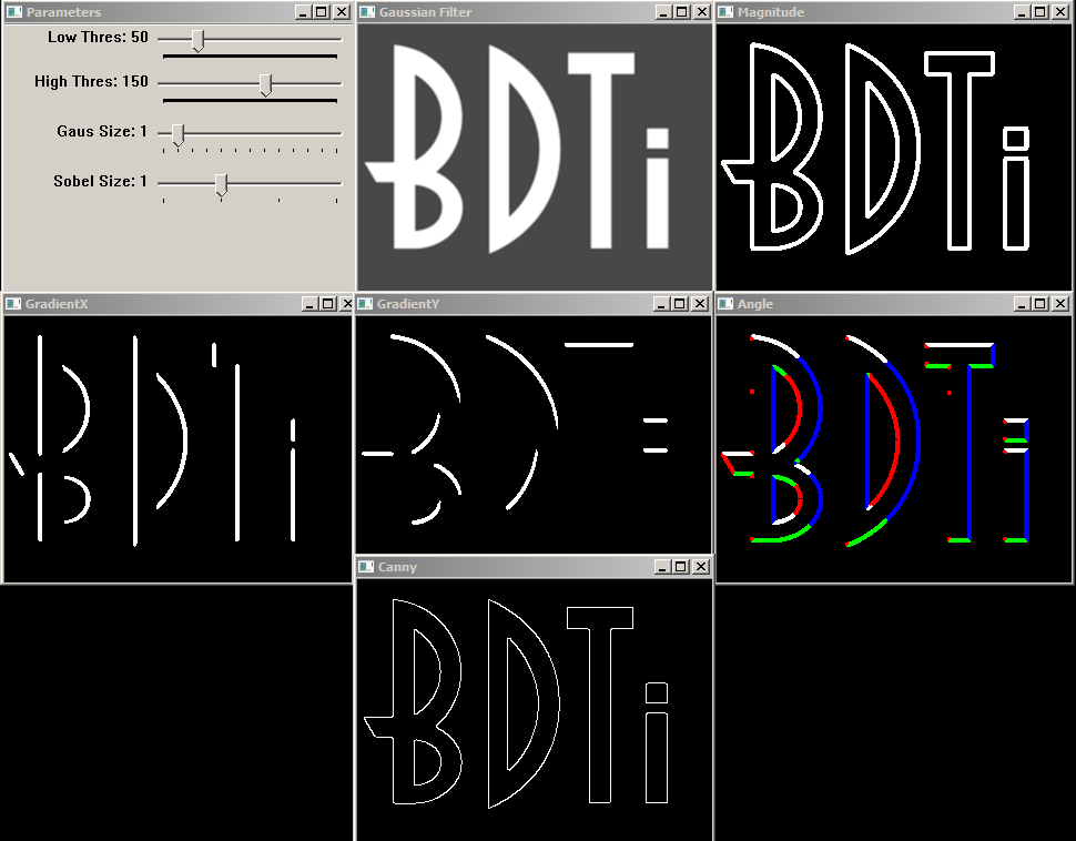
Figure 14. The user interface for the Canny edge detector example
The example allows you to modify the Canny parameters on the fly using simple slider controls.
Low Thres: Canny Low Threshold Parameter (T2) (LowThres)
High Thres: Canny High Threshold Parameter (T1) (HighThres)
Gaus Size : Gaussian Filter Size (Fsize)
Sobel Size: Sobel Operator Size (Ksize)
The example also opens six windows representing the stages in the Canny edge detection algorithm. All windows are updated in real-time.
Gaussian Filter: This window shows the output of the Gaussian filter.
GradientX: The result of the horizontal derivative (Sobel) of the image in the Gaussian Filter window.
GradientY: The result of the vertical derivative (Sobel) of the image in the Gaussian Filter window.
Magnitude: This window shows the result of combining the GradientX and GradientY images using the equation G = |Gx|+|Gy|
Angle: Color-coded result of the angle equation, combining GradientX and GradientY using arctan(Gy/Gx).
Black = 0 degrees
Red = 1 degrees to 45 degrees
White = 46 degrees to 135 degrees
Blue = 136 degrees to 225 degrees
Green = 226 degrees to 315 degrees
Red = 316 degrees to 359 degrees
The 0-degree marker indicates the left to right direction, as shown in figure 15.
Canny: The Canny edgemap

Figure 15. The Direction Color Code for the Angle Window in the Canny Edge Detector Example. Left to Right is 0 Degrees
Detection Time
Each of these examples writes the detection time to the console while the algorithm is running. This time represents the number of milliseconds the particular algorithm took to execute. A larger amount of time represents higher CPU utilization. The OpenCV library as built in these examples does not have hardware acceleration enabled; however OpenCV currently supports CUDA and NEON acceleration.
Conclusion
The intent of this article and accompanying BDTI Quick-Start OpenCV Kit software is to help the reader quickly get up and running with OpenCV. The examples discussed in this article represent only a miniscule subset of algorithms available in OpenCV; I chose them because at a high level they represent a broad variety of computer vision functions. Leveraging these algorithms in combination with, or alongside, other algorithms can help you solve various industrial, medical, automotive, and consumer electronics design problems.
About BDTI
Berkeley Design Technology, Inc. (BDTI) provides world-class engineering services for the design and implementation of complex, reliable, low-cost video and embedded computer vision systems. For details of BDTI technical competencies in embedded vision and a listing of example projects, go to www.BDTI.com.
For 20 years, BDTI has been the industry's trusted source of analysis, advice, and engineering for embedded processing technology and applications. Companies rely on BDTI to prove and improve the competitiveness of their products through benchmarking and competitive analysis, technical evaluations, and embedded signal processing software engineering. For free access to technology white papers, benchmark results for a wide range of processing devices, and presentations on embedded signal processing technology, visit www.BDTI.com.
Appendix: References
OpenCV v2.3 Programmer's Reference Guide
Viola-Jones Object Detector (PDF)
Good Features to Track (PDF)
Lucas-Kanade Optical Flow (PDF)
Revision History
| April 25, 2012 | Initial version of this document |
| May 3, 2012 | Added Canny edge detection example |