
This is a reprint of a Xilinx-published white paper which is also available here (1 MB PDF).
Xilinx INT8 optimization provide the best performance and most power efficient computational techniques for deep learning inference. Xilinx's integrated DSP architecture can achieve 1.75X solution-level performance at INT8 deep learning operations than other FPGA DSP architectures.
ABSTRACT
The intent of this white paper is to explore INT8 deep learning operations implemented on the Xilinx DSP48E2 slice, and how this contrasts with other FPGAs. With INT8, Xilinx's DSP architecture can achieve 1.75X peak solution-level performance at INT8 deep learning operation per second (OPS) compared to other FPGAs with the same resource count. As deep learning inference exploits lower bit precision without sacrificing accuracy, efficient INT8 implementations are needed.
Xilinx's DSP architecture and libraries are optimized for INT8 deep learning inference. This white paper describes how the DSP48E2 slice in Xilinx's UltraScale and UltraScale+ FPGAs can be used to process two concurrent INT8 multiply and accumulate (MACC) operations while sharing the same kernel weights. It also explains why 24-bit is the minimal size for an input to utilize this technique, which is unique to Xilinx. The white paper also includes an example of this INT8 optimization technique to show its relevance by revisiting the fundamental operations of neural networks.
INT8 for Deep Learning
Deep neural networks have propelled an evolution in machine learning fields and redefined many existing applications with new human-level AI capabilities. While more accurate deep learning models have been developed, their complexity is accompanied by high compute and memory bandwidth challenges. Power efficiency is driving innovation in developing new deep learning inference models that require lower compute intensity and memory bandwidth but must not be at the cost of accuracy and throughput. Reducing this overheard will ultimately increase power efficiency and lower the total power required.
In addition to saving power during computation, lower bit-width compute also lowers the power needed for memory bandwidth, because fewer bits are transferred with the same amount of memory transactions.
Research has shown that floating point computations are not required in deep learning inferences to keep the same level of accuracy1,2,3, and many applications, such as image classification, only require INT8 or lower fixed point compute precision to keep an acceptable inference accuracy2,3. Table 1 shows fine-tuned networks with dynamic fixed point parameters and outputs for convolutional and fully connected layers. The numbers in parentheses indicate accuracy without fine-tuning.
| Layer Outputs | CONV Parameters | FC Parameters | 32-Bit Floating Point Baseline | Fixed Point Accuracy | |
| LeNet (Exp1) | 4-bit | 4-bit | 4-bit | 99.1% | 99.0% (98.7%) |
| LeNet (Exp2) | 4-bit | 2-bit | 2-bit | 99.1% | 98.8% (98.0%) |
| Full CIFAR-10 | 8-bit | 8-bit | 8-bit | 81.7% | 81.4% (80.6%) |
| SqueezeNet top-1 | 8-bit | 8-bit | 8-bit | 57.7% | 57.1% (55.2%) |
|
CaffeNet top-1 |
8-bit | 8-bit | 8-bit | 56.9% | 56.0% (55.8%) |
| GoogLeNet top-1 | 8-bit | 8-bit | 8-bit | 68.9% | 66.6% (66.1%) |
Table 1: CNN Models with Fixed-Point Precision
Notes:
- Source: Gysel et al, Hardware-oriented Approximation of Convolutional Neural Networks, ICLR 20162
INT8 Deep Learning on Xilinx DSP Slices
Xilinx's DSP48E2 is designed to do one multiplication and addition operation, with up to 18×27 bit multiplication and up to 48-bits accumulation, efficiently within one clock cycle as shown in Figure 1. While looping back to itself or chaining multiple DSP slices together, multiplication and accumulation (MACC) can also be done efficiently with Xilinx devices.
Figure 1: DSP Slice with MACC Mode
While running INT8 computations, the wide 27-bit width is innately taken advantage of. In traditional applications, the pre-adder is usually utilized to implement (A+B) x C type of computations efficiently, but this type of computation is not very often seen in deep learning applications. Separating out the result of (A+B) x C into A x C and B x C, allows the accumulation in a separate dataflow, allowing it to fit a typical deep learning computation requirement.
Having an 18×27 bit multiplier is an advantage for INT8 deep learning operations. At a minimum one of the inputs to the multiplier needs to be at least 24-bits and the carry accumulator needs to be 32-bits to perform two INT8 MACC concurrently on one DSP slice. The 27-bit input can be combined with a 48-bit accumulator to achieve a 1.75X deep learning solution performance improvement (1.75:1 DSP multiplier to INT8 deep learning MACC ratio). FPGAs from other vendors only have an 18×19 multiplier in a single DSP block and are limited to a 1:1 ratio of DSP multiplier to INT8 MACC.
Scalable INT8 Optimization
The goal is to find a way to efficiently encode input a, b, and c so that the multiplication results between a, b and c can be easily separated into a x c and b x c.
In a reduced precision computation, e.g., INT8 multiplication, the higher 10-bit or 19-bit inputs are filled with 0s or 1s, and carry only 1-bit of information. This is also the same for the upper 29-bits of the final 45-bit product. Because of this, it is possible to use the higher 19-bits to carry another computation while the lower 8-bit and 16-bit input results are not affected.
Generally, two rules must be followed to utilize the unused upper bits for another computation:
- Upper bits should not affect the computation of the lower bits.
- Any contamination of the upper bits by the computation of the lower bits must be detectable and recoverable
To satisfy the above rules, the least significant bit of the upper product results must not fall into the lower 16-bits. Thus, the upper bits input should start with at least the 17th bit. For an 8-bit upper input that requires a minimum of 16 + 8 = 24-bits total input size. This minimum 24-bit input size can only guarantee two concurrent multiplications with one multiplier—but still not enough to reach the overall 1.75X MACC throughput.
Following are the steps to compute ac and bc in parallel in one DSP48E2 slice, which is used as an arithmetic unit with a 27-bit pre-adder (both inputs and outputs are 27-bits-wide) and a 27×18 multiplier. See Figure 2.
- Pack 8-bit input a and b in the 27-bit port p of the DSP48E2 multiplier via the pre-adder so that the 2-bit vectors are as far apart as possible.
The input a is left-shifted by only 18-bits so that two sign bits a in the 27-bit result from the first term to prevent overflow in the pre-adder when b<0 and a = –128. The shift amount for a being 18, or the width of the DSP48E2 multiplier port B, is coincidental.
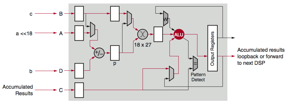
Figure 2: 8-Bit Optimization
- The DSP48E2 27×18 multiplier is used to compute the product of packed 27-bit port p and an 8-bit coefficient represented in 18-bit c in two's complement format. Now this 45-bit product is the sum of two 44-bit terms in two's complement format: ac left-shifted by 18-bits, and bc.
The post adder can be used to accumulate the above 45-bit product, which contains separable upper and lower product terms. Correct accumulations are carried for the upper and lower terms while accumulating the single 45-bit product. The final accumulation results, if not overflowed, can be separated by simple operations.
The limitation of this technique is the number of product terms each DSP slice can accumulate. With 2-bits remaining between the lower and upper product terms (Figure 3), accumulation of up to 7 product terms only can be guaranteed with no overflow for the lower bits. After 7 product terms, an additional DSP slice is required to extend this limitation. As a result, 8 DSP slices here perform 7×2 INT8 multiply-add operations, 1.75X the INT8 deep learning operations compared to competitive devices with the same number of multipliers.
There are many variations of this technique, depending on the requirements of actual use cases. Convolutional neural networks (CNN) with rectified linear unit (ReLU) produce non-negative activation, and the unsigned INT8 format creates one more bit of precision and 1.78X peak throughput improvement.
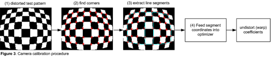
Figure 3: Packing Two INT8 Multiplication with a Single DSP48E2 Slice Compute Requirements for CNN
Compute Requirements for CNN
Modern neural networks are mostly derived from the original perceptron model4. See Figure 4.
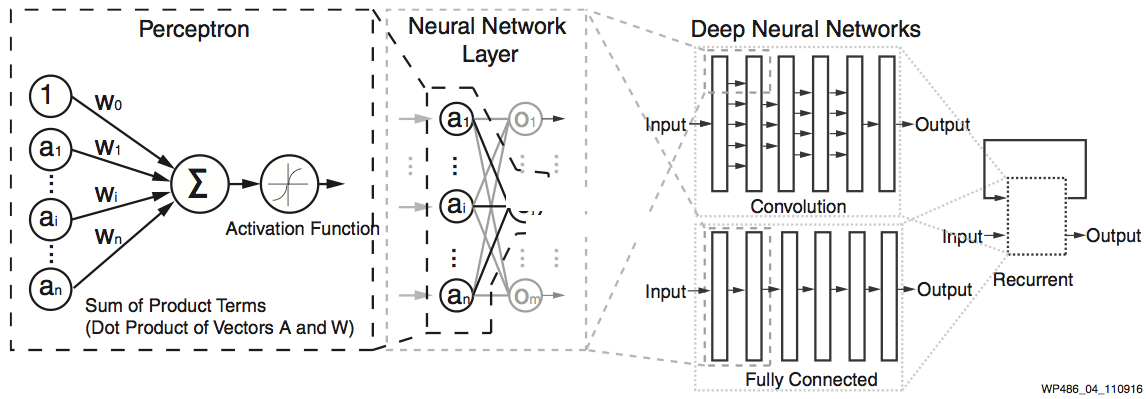
Figure 4: Perceptron and Deep Neural Networks
Although quite evolved from the standard perceptron structure, the basic operations of modern deep learning, also known as deep neural networks (DNN), are still perceptron-like operations, but in wider ensemble and deeper stacked perceptron structures. Figure 4 also shows the basic operation of a perceptron, through multiple layers, and ultimately repeated millions to billions of times in each typical deep learning inference. As shown in Figure 5, the major compute operations for computing each of the m perceptron/neuron outputs
oj (j∈[1,m])
in a layer of neural networks is: to take the entire n input samples
ai(i∈[1,n])
multiply each input by the corresponding kernel weight
wi,j(i∈[1,n]∈[1,m])
and accumulate the results
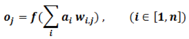
Where f(x) can be any activation function of choice.
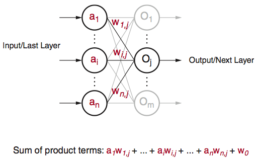
Figure 5: Perceptron in Deep Learning
If the precision of ai and wi,j are limited to INT8, this sum of products is the first of the parallel MACCs described in the INT8 optimization technique.
The second sum of the product uses the same input ai(i∈[1,n]), but a different set of kernel weights wi,k(i∈[1,n],k∈[1,m], and k≠j)
The result of the second perceptron/neuron output is
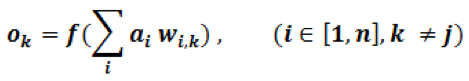
See Figure 6.
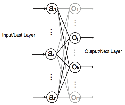
Figure 6: Two Sums of Product Terms in Parallel with Shared Input
By shifting the wi,k values 18-bits to the left using the INT8 optimization technique, each DSP slice results in a partial and independent portion of the final output values. The accumulator for each of the DSP slices is 48-bits-wide, and is chained to the next slice. This limits the number of chained blocks to 7, before saturation of the shifted wi,k affects the calculation, i.e., 2n MACCs with n DSP slices for the total of n input samples.
Each layer of a typical DNN has 100s to 1000s of input samples. However, after 7 terms of accumulation, the lower terms of the 48-bit accumulator might be saturated, and an extra DSP48E2 slice is needed for the summation every 7 terms. This equates to 14 MACCs with every 7 DSP slices plus one DSP slice for preventing the oversaturation, resulting in a throughout improvement of 7/4 or 1.75X.
In convolution neural networks (CNN), the same set of weights are usually reused heavily in convolutional layers, thus form a x w, and b x w type of parallel MACCs operations. So weight sharing instead of input sharing can also be used (see Figure 7).
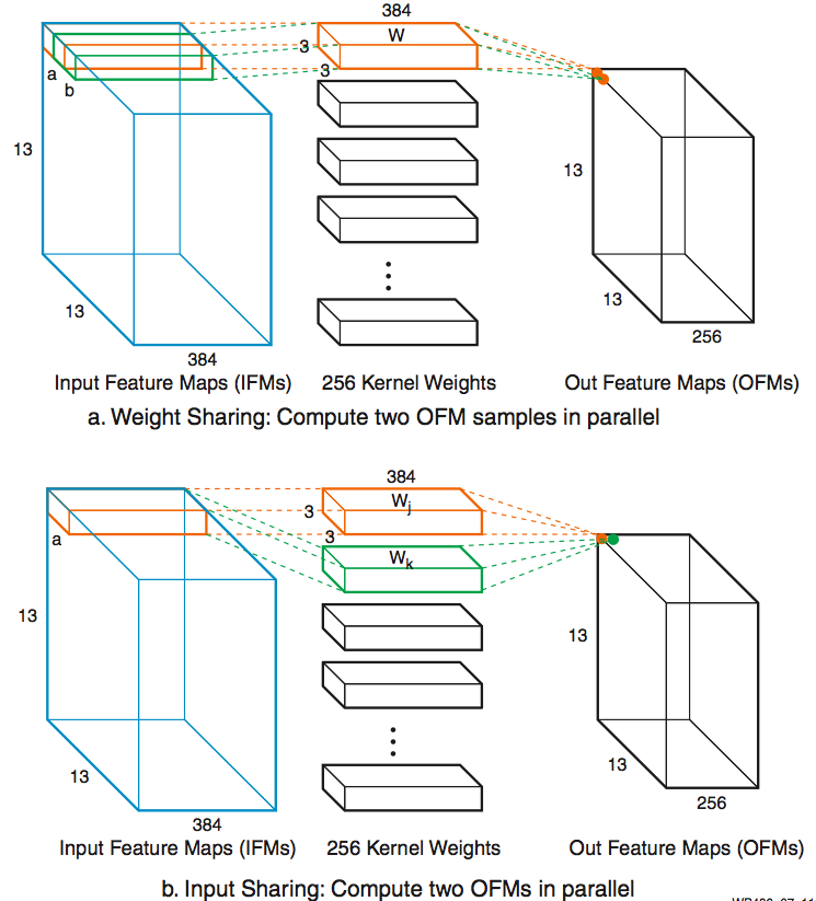
Figure 7: Weight Sharing and Input Sharing Comparison Other Methods to Create INT8 Chained MACCs
Other Methods to Create INT8 Chained MACCs
INT8 MACCs can also be constructed using the LUTs in the FPGA fabric at a similar frequency to the DSP slice. Depending on the usage of the FPGA, this could be a substantial increase in the deep learning performance, in some cases, increasing the performance by 3X. In many instances, with respect to other non-FPGA architectures, these available compute resources are not accounted for when calculating the available deep learning operations.
The programmable fabric in Xilinx FPGAs is unique because it can handle diverse workloads concurrently and efficiently. For example, Xilinx FPGAs can perform CNN image classification, networking cryptography, and data compression concurrently. Our deep-learning performance competitive analysis does not take the MACC LUTs into account because LUTs are usually more valuable while being used to perform other concurrent functions rather than to perform MACC functions.
Competitive Analysis
Intel’s (formerly Altera) Arria 10 and upcoming Stratix 10 devices are used in this competitive analysis against Xilinx's Kintex® UltraScale™ and Virtex® UltraScale+™ families. For this compute intensive comparison, the devices chosen have the highest DSP densities in each product family: Arria 10 (AT115), Stratix 10 (SX280), Kintex UltraScale (KU115), Virtex UltraScale+ (VU9P), and Virtex UltraScale+ (VU13P) devices. This comparison focuses on general-purpose MACC performance that can be used in many applications, such as deep learning.
Intel’s MACC performance is based on operators that leverage the pre-adders. However, this implementation produces the sum of product terms and not unique separate product terms—as such, Intel’s pre-adders are not suited for deep learning operations.
The power of Intel devices are estimated using Intel's EPE power estimate tools with the following worst-case assumptions:
- 90% DSP utilization at FMAX
- 50% logic utilization with clock rate at DSP FMAX
- 90% block RAM utilization with the clock rate at half DSP FMAX
- 4 DDR4 and 1 PCIe Gen3 x8
- 12.5% DSP toggle rate
- 80° TJ
Figure 8 shows the power efficiency comparison of deep learning operations. With INT8 optimization, Xilinx UltraScale and UltraScale+ devices can achieve 1.75X power efficiency on INT8 precision compared to INT16 operations (KU115 INT16 to KU115 INT8). And compared to Intel's Arria 10 and Stratix 10 devices, Xilinx devices deliver 2X–6X better power efficiency on deep learning inference operations.
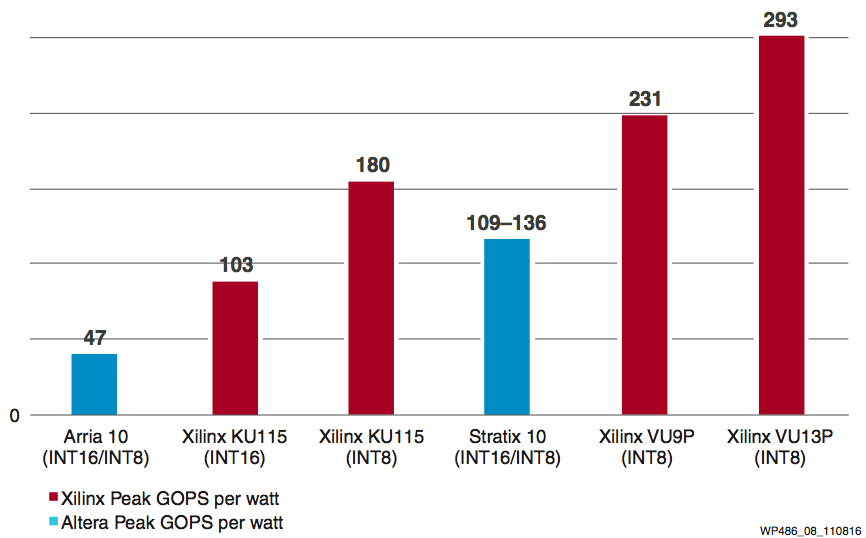
Figure 8: INT8 Deep Learning Power Efficiency Comparison: Xilinx vs. Intel
Conclusion
This white paper explores how INT8 deep learning operations are optimal on Xilinx DSP48E2 slices, achieving a 1.75X performance gain. The Xilinx DSP48E2 slice can be used to do concurrent INT8 MACCs while sharing the same kernel weights. To implement INT8 efficiently, an input width of 24-bits is required, an advantage that is only supported in Xilinx UltraScale and UltraScale+ FPGA DSP slices. Xilinx is well suited for INT8 workloads for deep learning applications (e.g., image classification). Xilinx is continuing to innovate new hardware- and software-based methodologies to accelerate deep learning applications.
For more information on deep learning in the data center, go to:
https://www.xilinx.com/accelerationstack
References
- Dettmers, 8-Bit Approximations for Parallelism in Deep Learning, ICLR 2016
https://arxiv.org/pdf/1511.04561.pdf - Gysel et al, Hardware-oriented Approximation of Convolutional Neural Networks, ICLR 2016
https://arxiv.org/pdf/1604.03168v3.pdf - Han et al, Deep Compression: Compressing Deep Neural Networks With Pruning, Trained Quantization And Huffman Coding, ICLR 2016
https://arxiv.org/pdf/1510.00149v5.pdf - Rosenblatt, F., The Perceptron: A Probabilistic Model for Information Storage and Organization in the Brain, Psychological Review, Vol. 65, No. 6, 1958
http://www.ling.upenn.edu/courses/cogs501/Rosenblatt1958.pdf
By: Yao Fu, Ephrem Wu, Ashish Sirasao, Sedny Attia, Kamran Khan, and Ralph Wittig